Structural design of concrete 3D discontinuities in IDEA StatiCa Detail

Introduction to the 3D CSFM method

General introduction for the structural design of concrete 3D details
Main assumptions and limitations
Mohr-Coulomb plasticity theory implementation in 3D CSFM
General mechanics assumptions for 3D CSFM

Analysis model of IDEA StatiCa 3D Detail

Introduction to finite element implementation
Finite element types
Load transfer devices
Meshing in 3D CSFM
Solution method and load-control algorithm for 3D CSFM
Presentation of 3D results
Model imported from IDEA StatiCa Connection

Model verification

Limit states

Structural verifications according to EUROCODE

- Material models in 3D CSFM (EN)
- Partial safety factors
- Ultimate limit state checks

Structural verifications according to ACI 318-19

- Material models in 3D CSFM (ACI)
- Strength reduction and load factors
- Strength verifications

Introduction to the 3D CSFM method

Analysis model of IDEA StatiCa 3D Detail

Model verification

Structural verifications according to EUROCODE

Structural verifications according to ACI 318-19

3D CSFM is in accordance with ACI 318-19, chapter 6.8.1.1. In order for the 3D CSFM to meet the requirements from ACI 318-19 Section 6.8.1.2, a lot of verification testing was done at various universities. Individual articles summarizing the results of verification and validation can be found at the following link.

• Verifications: Detail 3D

Material models (EN)

Concrete - ULS

The concrete model implemented in the CSFM is based on the uniaxial compression constitutive laws prescribed by EN 1992-1-1 for the design of cross-sections, which only depend on compressive strength. The parabola-rectangle diagram specified in EN 1992-1-1 (Fig. 26a) is used by default in the CSFM, but designers can also choose a more simplified elastic ideal plastic relationship (Fig. 26b). The tensile strength is neglected, as it is in classic reinforced concrete design.

\[ \textsf{\textit{\footnotesize{Fig. 26\qquad The stress-strain diagrams of concrete for ULS: a) parabola-rectangle diagram; b) bilinear diagram.}}}\]

Using default settings, the current implementation of the CSFM in IDEA StatiCa Detail does not consider an explicit failure criterion in terms of strains for concrete in compression (i.e., after the peak stress is reached it considers a plastic branch with ε_cu2 (ε_cu3) in value 5% while EN 1992-1-1 assumes ultimate strain less than 0,35%). This simplification does not allow the deformation capacity of structures failing in compression to be verified. However, their ultimate capacity is properly predicted when, in addition to the factor of cracked concrete (k_c2 defined in (Fig. 27)), the increase in the brittleness of concrete as its strength rises is considered by means of the \(\eta_{fc}\) reduction factor defined in fib Model Code 2010 as follows:

\[f_{cd}=\frac{f_{ck,red}}{γ_c} = \frac{k_c \cdot f_{ck}}{γ_c} = \frac{\eta _{fc} \cdot k_{c2} \cdot f_{ck}}{γ_c}\]

\[{\eta _{fc}} = {\left( {\frac{{30}}{{{f_{ck}}}}} \right)^{\frac{1}{3}}} \le 1\]

where:

k_c is the global reduction factor of the compressive strength

k_c2 is the reduction factor due to the presence of transverse cracking

f_ck is the concrete cylinder characteristic strength (in MPa for the definition of \( \eta_{fc} \)).

\[ \textsf{\textit{\footnotesize{Fig. 27\qquad The compression softening law.}}}\]

Concrete - SLS

The serviceability analysis contains certain simplifications of the constitutive models which are used for ultimate limit state analysis. A perfect bond is assumed, i.e., the anchorage length is not verified at serviceability. Furthermore, the plastic branch of the stress-strain curve of concrete in compression is disregarded, while the elastic branch is linear and infinite. Compression softening law is not considered. These simplifications enhance the numerical stability and calculation speed and do not reduce the generality of the solution as long as the resultant material stress limits at serviceability are clearly below their yielding points (as required by Eurocode). Therefore, the simplified models used for serviceability are only valid if all verification requirements are fulfilled.

\[ \textsf{\textit{\footnotesize{Fig. 28\qquad Concrete stress-strain diagrams implemented for serviceability analysis: short- and long-term verifications.}}}\]

Long term effects

In serviceability analysis, the long-term effects of concrete are considered using an effective infinite creep coefficient (\(\varphi\), taken as a value of 2.5 by default) which modifies the secant modulus of elasticity of concrete (E_cm) as follows:

\[E_{c,eff} = \frac{E_{cm}}{1+\varphi}\]

When considering long-term effects, a load step with all permanent loads is first calculated considering the creep coefficient (i.e., using the effective modulus of elasticity of concrete, E_c,eff) and, then, the additional loads are calculated without the creep coefficient (i.e., using E_cm). In addition, to conduct short-term verifications, another calculation is performed in which all loads are calculated without the creep coefficient. Both calculations for long and short-term verifications are depicted in Fig. 28.

Reinforcement

By default, the idealized bilinear stress-strain diagram for the bare reinforcing bars typically defined by design codes (Fig. 29) is considered. The definition of this diagram only requires basic properties of the reinforcement to be known during the design phase (strength and ductility class). Whenever known, the actual stress-strain relationship of the reinforcement (hot-rolled, cold-worked, quenched and self-tempered, …) can be considered. The reinforcement stress-strain diagram can be defined by the user, but in this case, it is impossible to assume tension stiffening effect (it is impossible to calculate crack width). Using the stress-strain diagram with horizontal top branch does not allow to the verification of structural durability. Therefore, manual verification of standard ductility requirements is necessary.

\( \textsf{\textit{\footnotesize{Fig. 29 \qquad Stress-strain diagram of reinforcement: a) bilinear diagram with an inclined top branch; b) bilinear diagram}}}\) \( \textsf{\textit{\footnotesize{with a horizontal top branch.}}}\)

Tension stiffening (Fig. 30)  is accounted for automatically by modifying the input stress-strain relationship of the bare reinforcing bar in order to capture the average stiffness of the bars embedded in the concrete (ε_m), following the approaches presented in Section 1.2.4.

\[ \textsf{\textit{\footnotesize{Fig. 30\qquad Scheme of tension stiffening.}}}\]

Safety factors

The Compatible Stress Field Method is compliant with modern design codes. As the calculation models only use standard material properties, the partial safety factor format prescribed in the design codes can be applied without any adaptation. In this way, the input loads are factored, and the characteristic material properties are reduced using the respective safety coefficients prescribed in design codes, exactly as in conventional concrete analysis. Values of material safety factors prescribed in EN 1992-1-1 chap. 2.4.2.4 are set by default, but user can change safety factors in Setup (Fig. 31).

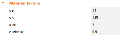
\[ \textsf{\textit{\footnotesize{Fig. 31\qquad The setting of  material safety factors in Idea StatiCa Detail.}}}\]

Load safety factors has to be defined by user in Combination rule for each non-linear combination of load cases (Fig. 32). For all templates implemented in Idea StatiCa Detail, partial safety factors are already predefined.

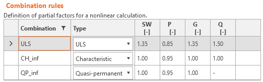
\[ \textsf{\textit{\footnotesize{Fig. 32\qquad The setting of  load partial factors in Idea StatiCa Detail.}}}\]

By using appropriate user-defined combinations of partial safety factors, users can also compute with the CSFM using the global resistance factor method (Navrátil, et al. 2017), but this approach is hardly ever used in design practice. Some guidelines recommend using the global resistance factor method for non-linear analysis. However, in simplified non-linear analyses (such as the CSFM), which only require those material properties that are used in conventional hand calculations, it is still more desirable to use the partial safety format.

Ultimate limit state analysis

The different verifications required by EN 1992-1-1 are assessed based on the direct results provided by the model. ULS verifications are carried out for concrete strength, reinforcement strength, and anchorage (bond shear stresses).

The concrete strength in compression is evaluated as the ratio between the maximum principal compressive stress σ_c3 obtained from FE analysis and the limit value σ_c3,lim. Then:

\[\frac{σ_{c3}}{σ_{c3,lim}}\]

\[σ_{c3,lim} = f_{cd} = α_{cc} \cdot \frac{f_{ck,red}}{γ_c} = α_{cc} \cdot \frac{k_c \cdot f_{ck}}{γ_c} = α_{cc} \cdot \frac{\eta _{fc} \cdot k_{c2} \cdot f_{ck}}{γ_c}\]

\[{\eta _{fc}} = {\left( {\frac{{30}}{{{f_{ck}}}}} \right)^{\frac{1}{3}}} \le 1\]

where:

f_ck        characteristic cylinder strength of concrete,

k_c2       compression softening factor (see 5.1.1),

γ_c             is the partial safety factor for concrete, γ_c = 1,5,

α_cc       is the coefficient taking account of long term effects on the compressive strength and of unfavourable effects resulting from the way the load is applied. The default value is 1,0.

The strength of the reinforcement is evaluated in both tension and compression as the ratio between the stress in the reinforcement at the cracks σ_sr and the specified limit value σ_sr,lim:

\[\frac{σ_{sr}}{σ_{sr,lim}}\]

\(σ_{c3,lim} = \frac{k \cdot f_{yk}}{γ_s}\qquad\qquad\textsf{\small{for bilinear diagram with inclined top branch}}\)

\(σ_{c3,lim} = \frac{f_{yk}}{γ_s}\qquad\qquad\,\,\,\,\textsf{\small{for bilinear diagram with horizontal top branch}}\)

where:

f_yk        yield strength of the reinforcement,

k          the ratio of tensile strength f_tk to the yield stress,
            \(k = \frac{f_{tk}}{f_{yk}}\)

γ_s             is the partial safety factor for reinforcement γ_s = 1,15.

The bond shear stress is evaluated independently as the ratio between the bond stress τ_b calculated by FE analysis and the ultimate bond strength f_bd, according to EN 1992-1-1 chap. 8.4.2:

\[\frac{τ_{b}}{f_{bd}}\]

\[f_{bd} = 2.25 \cdot η_1\cdot η_2\cdot f_{ctd}\]

where:

 f_ctd      is the design value of concrete tensile strength. Due to the increasing brittleness of higher strength concrete, f_ctk,0,05 is limited to the value for C60/75,

 η₁       is a coefficient related to the quality of the bond condition and the position of the bar during concreting (Fig. 33):

             η₁ = 1,0 when ‘good’ conditions are obtained and

             η₁ = 0,7 for all other cases and for bars in structural elements built with slip-forms, unless it can be shown that ‘good’ bond conditions exist

η₂        is related to the bar diameter:

            η₂ = 1,0 for Ø ≤ 32 mm

            η₂ = (132 - Ø)/100 for Ø > 32 mm

\[ \textsf{\textit{\footnotesize{Fig. 33\qquad Description of bond conditions.}}}\]

These verifications are carried out with respect to the appropriate limit values for the respective parts of the structure (i.e., in spite of having a single grade both for concrete and reinforcement material, the final stress-strain diagrams will differ in each part of the structure due to tension stiffening and compression softening effects).

Verifications and validations

• Verifications: Detail 3D

References

1. Wu, D.; Wang, Y.; Qiu, Y.; Zhang, J.; Wan, Y.-K. Determination of Mohr–Coulomb Parameters from Nonlinear Strength Criteria for 3D Slopes. Math. Probl. Eng. 2019, 6927654.
2. Lelovic, S.; Vasovic, D.; Stojic, D. Determination of the Mohr-Coulomb Material Parameters for Concrete under Indirect Tensile Test. Tech. Gaz. 2019, 26, 412–419.
3. Galic, M.; Marovic, P.; Nikolic, Ž. Modified Mohr-Coulomb—Rankine material model for concrete. Eng. Comput. 2011, 28, 853–887.
4. Fan, Q.; Gu, S.C.; Wang, B.N.; Huang, R.B. Two Parameter Parabolic Mohr Strength Criterion Applied to Analyze The Results of the Brazilian Test. Appl. Mech. Mater. 2014, 624, 630–634.